


股市趨勢預測對投資者和數據科學家來說都是一个重大的挑戰,因為市場的波動性和複雜性。然而,隨著機器學習(ML)的出現,现在已经可以開發出分析歷史數據並提供對潛在未來趨勢洞察的預測模型。在這個全面的指南中,我們將探索如何使用Python和機器學習有效地預測股價和市場趨勢。
1. 問題概述
股市受到多種因素的影響,包括:
-
宏观經濟指標(如通脹、GDP、失業率)
-
公司基本面(盈利、收入、市盈率)
-
市場情緒(新聞文章、社交媒體活動)
-
技術因素(價格行動、移動平均線、成交量趨勢)
股市的不確定性非常高,沒有任何模型能提供完美的預測。然而,透過分析歷史價格數據和技術指標,我們可以提取有助于預測未來價格趨勢的模式,例如股票在短期或長期內會升值還是貶值。
2. 收集股市數據
建立預測股票模型的第一步是收集歷史股票數據。這些數據可從財務數據提供商那裡輕鬆獲得,例如:
-
Yahoo 財經(通過
yfinancePython套件) -
Quandl
-
Alpha Vantage
使用yfinance,您可以下載歷史股票數據。讓我們抓取過去十年蘋果公司(AAPL)的數據。
pip install yfinance
import yfinance as yf

# Fetch data for Apple (AAPL) from Yahoo Finance
data = yf.download('AAPL', start='2024-01-01', end='2024-04-01')
print(data.head())  # View the first few rows of the dataset
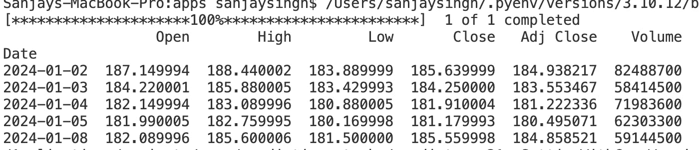
這些數據包含了一些重要列,如:
-
Open:當天開盤價格
-
High:當天最高價格
-
Low:當天最低價格
-
關閉
: 當日收市價格
-
成交量: 當日成交股數
-
調整後收市: 考慮紅利和分割的調整後收市價格
3. 特徵工程
特徵工程在機器學習中至關重要。它涉及從現有數據中創造新特徵,以提升模型的預測能力。在股市預測方面,一些最常用的特徵是技術指標。
常見技術指標:
-
簡單移動平均(SMA): 通過取特定期數的給定價格的算術平均值來計算移動平均。
-
指數移動平均(EMA): 一個給 recent price data 較高權重的加权移動平均。
-
相關強度指數(RSI)
: 一種動力震盪器,用以量大宗商品價格移動的速度和變化。
-
移动平均收敛发散指标(MACD): 一种趋势跟踪的动量指标,显示股票价格的两个移动平均线之间的关系。
-
布林带: 一种波动性指标,包括一个中间带(SMA)和两个外侧带(标准差)。
以下是您如何在Python中计算这些技术指标的方法:
# Calculate Simple Moving Averages (SMA)
data['SMA_20'] = data['Close'].rolling(window=20).mean()
data['SMA_50'] = data['Close'].rolling(window=50).mean()

# Calculate Exponential Moving Averages (EMA)
data['EMA_20'] = data['Close'].ewm(span=20, adjust=False).mean()

# Calculate Relative Strength Index (RSI)
delta = data['Close'].diff(1)
gain = delta.where(delta > 0, 0)
loss = -delta.where(delta < 0, 0)
avg_gain = gain.rolling(window=14).mean()
avg_loss = loss.rolling(window=14).mean()
rs = avg_gain / avg_loss
data['RSI'] = 100 - (100 / (1 + rs))

# Drop rows with NaN values
data = data.dropna()
您包含的技术指标越多,您的数据集就越丰富,用于训练机器学习模型的效果越好。但是,请确保您所选择的指标与您的预测任务相关。
4. 为机器学习准备数据集
既然您已经创建了您的技术指标,您必须通过将其分为特征(X)和目标(y)来准备数据集。目标是您想要预测的变量(例如,下一天的收盘价)。以下是您可以如何设置:
# Define the target variable as the next day's closing price
data['Target'] = data['Close'].shift(-1)

# Drop the last row, which has NaN in the 'Target' column
data = data.dropna(subset=['Target'])

# Feature set (dropping unnecessary columns)
X = data[['SMA_20', 'SMA_50', 'EMA_20', 'RSI']]
y = data['Target']

# Drop rows with missing values
X = X.dropna()
y = y[X.index]  # Ensure target variable aligns with features
接下來的步驟是將數據分割為訓練集和測試集,以評估模型的性能:
from sklearn.model_selection import train_test_split

# Split into training and testing data
X_train, X_test, y_train, y_test = train_test_split(X, y, test_size=0.2, random_state=42)
5. 選擇和訓練一個機器學習模型
對於股市預測,可以使用的多篇機器學習算法包括:
-
線性迴歸:基於變量之間的關係進行預測的簡單模型。
-
隨機森林:能夠處理非線性關係並且抗過擬合能力较强的多功能模型。
-
支持向量機 (SVM):對於分類和回歸任務都很有用。
-
長短期記憶網絡 (LSTM):特別適合時間序列數據的一種神經網絡。
為了簡化,讓我們從一個隨機森林回歸器開始,它是一個強大的集成學習算法:
from sklearn.ensemble import RandomForestRegressor
from sklearn.metrics import mean_squared_error

# Initialize and train the model
model = RandomForestRegressor(n_estimators=100, random_state=42)
model.fit(X_train, y_train)

# Predict on the test set
y_pred = model.predict(X_test)

# Evaluate the model using Mean Squared Error (MSE)
mse = mean_squared_error(y_test, y_pred)
print(f"Mean Squared Error: {mse}")
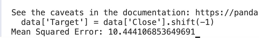
6. 模型評估
均方誤差(MSE)有助於衡量模型的預測誤差。MSE愈低,模型的預測能力愈好。為了視覺化模型對股票價格的預測效果,可以繪製實際價格與預測價格的對比圖:
import matplotlib.pyplot as plt
# Plot actual vs predicted prices
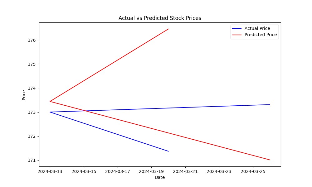
plt.figure(figsize=(10, 6))
plt.plot(y_test.index, y_test, label='Actual Price', color='blue')
plt.plot(y_test.index, y_pred, label='Predicted Price', color='red')
plt.title('Actual vs Predicted Stock Prices')
plt.xlabel('Date')
plt.ylabel('Price')
plt.legend()
plt.show()
這張圖將幫助你視覺化評估模型的表現,顯示預測值與實際股票價格的接近程度。
完整代碼:
import matplotlib.pyplot as plt
from sklearn.metrics import mean_squared_error
from sklearn.ensemble import RandomForestRegressor
from sklearn.model_selection import train_test_split
import yfinance as yf

# Fetch data for Apple (AAPL) from Yahoo Finance
data = yf.download('AAPL', start='2024-01-01', end='2024-04-01')
print(data.head())  # View the first few rows of the dataset

# Calculate Simple Moving Averages (SMA)
data['SMA_20'] = data['Close'].rolling(window=20).mean()
data['SMA_50'] = data['Close'].rolling(window=50).mean()

# Calculate Exponential Moving Averages (EMA)
data['EMA_20'] = data['Close'].ewm(span=20, adjust=False).mean()

# Calculate Relative Strength Index (RSI)
delta = data['Close'].diff(1)
gain = delta.where(delta > 0, 0)
loss = -delta.where(delta < 0, 0)
avg_gain = gain.rolling(window=14).mean()
avg_loss = loss.rolling(window=14).mean()
rs = avg_gain / avg_loss
data['RSI'] = 100 - (100 / (1 + rs))

# Drop rows with NaN values (due to moving averages and RSI)
data = data.dropna()

# Define the target variable as the next day's closing price
data['Target'] = data['Close'].shift(-1)

# Drop the last row, which has NaN in the 'Target' column
data = data.dropna(subset=['Target'])

# Feature set (SMA, EMA, RSI)
X = data[['SMA_20', 'SMA_50', 'EMA_20', 'RSI']]
y = data['Target']

# Split into training and testing data
X_train, X_test, y_train, y_test = train_test_split(
    X, y, test_size=0.2, random_state=42)

# Initialize and train the model
model = RandomForestRegressor(n_estimators=100, random_state=42)
model.fit(X_train, y_train)

# Predict on the test set
y_pred = model.predict(X_test)

# Evaluate the model using Mean Squared Error (MSE)
mse = mean_squared_error(y_test, y_pred)
print(f"Mean Squared Error: {mse}")


# Plot actual vs predicted prices
plt.figure(figsize=(10, 6))
plt.plot(y_test.index, y_test, label='Actual Price', color='blue')
plt.plot(y_test.index, y_pred, label='Predicted Price', color='red')
plt.title('Actual vs Predicted Stock Prices')
plt.xlabel('Date')
plt.ylabel('Price')
plt.legend()
plt.show()
7. 提升模型
現在你已經建立了基本模型,有許多方法可以提升其準確度:
-
使用額外特徵:包含更多技術指標,新聞和社交媒體的情感分析數據,甚至是宏觀經濟變量。
-
進階機器學習模型:嘗試更複雜的演算法,如XGBoost,梯度提升機器(GBM),或是深度學習模型如LSTM,以改進時間序列數據的表現。
-
超參數調整
: 使用GridSearchCV 或 RandomSearchCV等技術來優化模型參數,以找到最佳模型配置。
- 特徵選擇: 使用如遞歸特徵消除 (RFE)的技術來識別對預測有最重要貢獻的特徵。
Conclusion
通過不斷優化您的模型、加入更多數據以及嘗試不同的算法,您可以提高您的股市趨勢預測模型的預測能力。
下一步
-
嘗試使用更多的技術指標和數據來源。
-
嘗試不同的機器學習算法(例如,為深度學習使用LSTM)。
-
通過使用歷史數據模擬交易來回测您的模型。
-
根據real-world performance的回饋持續優化及調整您的模型。
Source:
https://blog.bytescrum.com/how-to-predict-stock-market-trends-with-python-and-machine-learning