


株の市場の动向予測は、市場の変動や複雑さにより、投資家とデータ科学者どおりにとって重要な挑戦をもたらしています。しかし、機械学習(ML)の到来により、過去のデータを分析し、未来の動向についての洞察を提供する予測モデルの開発が可能になりました。この完全なガイドで、あなたがどのようにPythonと機械学習を使用して株価と市場の動向を効果的に予測するかを探ります。
1. 問題の概要
株市場は、以下のような複数の要因に影響されます。
-
マクロ経済指標(インフレ、GDP、失業率など)
-
会社の基本面(収益、売上、PERatio)
-
市場的情報(ニュース記事、ソーシャルメディアの活動)
-
技術的な要因(価格行動、移動平均、量の趨勢)
株式市場における高い不確実性を考慮しても、完璧な予測はできない model です。しかし、過去の価格データと技術的指標を分析することで、株の価値が短期間や長期间にどのように変動するかを予測するためのパターンを抽出することができます。
2. 株市場のデータの収集
予測的な株のモデルを構築するための最初のステップは、過去の株のデータを収集することです。このデータは、金融データ提供者からすぐに利用できます。
-
Yahoo Finance (
yfinancePython パッケージを使用して) -
Quandl
-
Alpha Vantage
yfinance を使用して、過去の株のデータをダウンロードすることができます。過去10年間のアップル (AAPL) のデータを取得してみましょう。
pip install yfinance
import yfinance as yf

# Fetch data for Apple (AAPL) from Yahoo Finance
data = yf.download('AAPL', start='2024-01-01', end='2024-04-01')
print(data.head())  # View the first few rows of the dataset
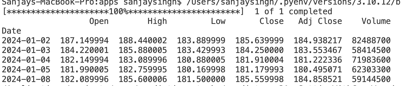
このデータには、必要な列が含まれています。
-
Open: その日の始値
-
High: その日の最高値
-
Low: その日の最低値
-
終値
: 当日の終値
-
成交量: 当日の取引された株数
-
調整後の終値: 配当と分割を考慮した調整後の終値
3. 特徴 engineering
特徴 engineeringは機械学習において非常に重要であり、既存のデータから新しい特徴を作成することでモデルの予測能力を高めることができます。株の予測においては、最も一般的に使用される特徴の1つに技術指標があります。
一般的な技術指標:
-
単純移動平均(SMA): 特定の期间数の価格の算術平均を計算した移動平均をいいます。
-
指数移動平均(EMA): 最近の価格データにより重みを与えた移動平均です。
-
相対強度指標(RSI)
:価格の動きのスピードと変化を計る動量周波数観測器。
-
動的平均聚合分散(MACD):株の価格の2つの動的平均間の関係を示すトレンド追求の動量指標。
-
ボリンジャー带:中央の帯(SMA)と2つの外側の帯(標準偏差)を含む変動性指標。
これらの技術的指標をPythonで計算する方法は以下の通りです:
# Calculate Simple Moving Averages (SMA)
data['SMA_20'] = data['Close'].rolling(window=20).mean()
data['SMA_50'] = data['Close'].rolling(window=50).mean()

# Calculate Exponential Moving Averages (EMA)
data['EMA_20'] = data['Close'].ewm(span=20, adjust=False).mean()

# Calculate Relative Strength Index (RSI)
delta = data['Close'].diff(1)
gain = delta.where(delta > 0, 0)
loss = -delta.where(delta < 0, 0)
avg_gain = gain.rolling(window=14).mean()
avg_loss = loss.rolling(window=14).mean()
rs = avg_gain / avg_loss
data['RSI'] = 100 - (100 / (1 + rs))

# Drop rows with NaN values
data = data.dropna()
技術的指標を多く含めることで、機械学習モデルのトレーニング用のデータセットが豊富になります。しかし、選択した指標は、予測タスクに関連していることを確認してください。
4. 機械学習のためのデータセット準備
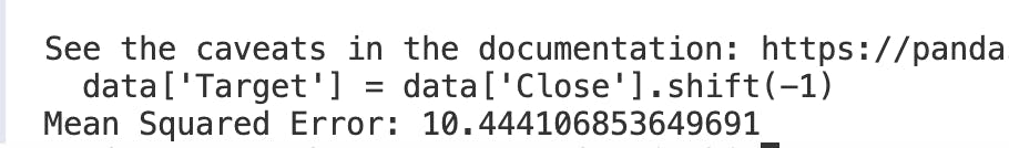
技術的指標を作成した後、特徴(X)と目的変数(y)に分割してデータセットを準備する必要があります。目的変数は、次の日の終値を予測したい変数です。以下はこれを設定する方法です。
# Define the target variable as the next day's closing price
data['Target'] = data['Close'].shift(-1)

# Drop the last row, which has NaN in the 'Target' column
data = data.dropna(subset=['Target'])

# Feature set (dropping unnecessary columns)
X = data[['SMA_20', 'SMA_50', 'EMA_20', 'RSI']]
y = data['Target']

# Drop rows with missing values
X = X.dropna()
y = y[X.index]  # Ensure target variable aligns with features
次に、データを訓練集とテスト集に分割して、モデルの性能を評価する:
from sklearn.model_selection import train_test_split

# Split into training and testing data
X_train, X_test, y_train, y_test = train_test_split(X, y, test_size=0.2, random_state=42)
5. 機械学習モデルの選択とトレーニング
株市場の予測には、以下のようないくつかの機械学習アルゴリズムが使用できます:
-
線形回帰:変数間の関係に基づいて予測する簡単なモデル。
-
ランダム森林:非線形関係や过学習を良く处理できる汎用性のあるモデル。
-
サポートベクタマシン(SVM):分类と回帰の両方のタスクに有用。
-
長短期記憶(LSTM):時間序列データに特に適したニューラルネットワークの一型。
単純性のために、ランダム森林レグレッサー、強力な集合学習アルゴリズムを始めましょう:
from sklearn.ensemble import RandomForestRegressor
from sklearn.metrics import mean_squared_error

# Initialize and train the model
model = RandomForestRegressor(n_estimators=100, random_state=42)
model.fit(X_train, y_train)

# Predict on the test set
y_pred = model.predict(X_test)

# Evaluate the model using Mean Squared Error (MSE)
mse = mean_squared_error(y_test, y_pred)
print(f"Mean Squared Error: {mse}")
6. モデル評価
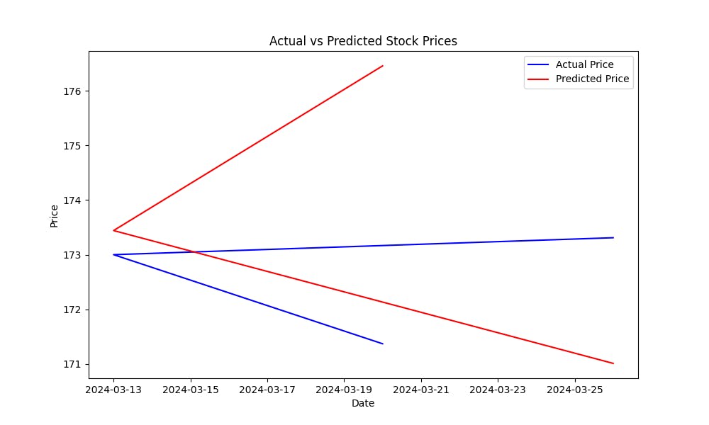
平均二乗誤差(MSE)は、モデルの予測誤差を衡量するのに役立ちます。MSEが低いと、モデルの予測が良いことを示します。モデルが株の価格を予測する能力を視覚的に確認するために、実際の価格と予測価格をプロットします:
import matplotlib.pyplot as plt

# Plot actual vs predicted prices
plt.figure(figsize=(10, 6))
plt.plot(y_test.index, y_test, label='Actual Price', color='blue')
plt.plot(y_test.index, y_pred, label='Predicted Price', color='red')
plt.title('Actual vs Predicted Stock Prices')
plt.xlabel('Date')
plt.ylabel('Price')
plt.legend()
plt.show()
このプロットは、予測値が実際の株価格にどれだけ近いかを示していることがわかりやすく、モデルの性能を視覚的に評価するのに役立つかもしれません。
コード全体:
import matplotlib.pyplot as plt
from sklearn.metrics import mean_squared_error
from sklearn.ensemble import RandomForestRegressor
from sklearn.model_selection import train_test_split
import yfinance as yf

# Fetch data for Apple (AAPL) from Yahoo Finance
data = yf.download('AAPL', start='2024-01-01', end='2024-04-01')
print(data.head())  # View the first few rows of the dataset

# Calculate Simple Moving Averages (SMA)
data['SMA_20'] = data['Close'].rolling(window=20).mean()
data['SMA_50'] = data['Close'].rolling(window=50).mean()

# Calculate Exponential Moving Averages (EMA)
data['EMA_20'] = data['Close'].ewm(span=20, adjust=False).mean()

# Calculate Relative Strength Index (RSI)
delta = data['Close'].diff(1)
gain = delta.where(delta > 0, 0)
loss = -delta.where(delta < 0, 0)
avg_gain = gain.rolling(window=14).mean()
avg_loss = loss.rolling(window=14).mean()
rs = avg_gain / avg_loss
data['RSI'] = 100 - (100 / (1 + rs))

# Drop rows with NaN values (due to moving averages and RSI)
data = data.dropna()

# Define the target variable as the next day's closing price
data['Target'] = data['Close'].shift(-1)

# Drop the last row, which has NaN in the 'Target' column
data = data.dropna(subset=['Target'])

# Feature set (SMA, EMA, RSI)
X = data[['SMA_20', 'SMA_50', 'EMA_20', 'RSI']]
y = data['Target']

# Split into training and testing data
X_train, X_test, y_train, y_test = train_test_split(
    X, y, test_size=0.2, random_state=42)

# Initialize and train the model
model = RandomForestRegressor(n_estimators=100, random_state=42)
model.fit(X_train, y_train)

# Predict on the test set
y_pred = model.predict(X_test)

# Evaluate the model using Mean Squared Error (MSE)
mse = mean_squared_error(y_test, y_pred)
print(f"Mean Squared Error: {mse}")


# Plot actual vs predicted prices
plt.figure(figsize=(10, 6))
plt.plot(y_test.index, y_test, label='Actual Price', color='blue')
plt.plot(y_test.index, y_pred, label='Predicted Price', color='red')
plt.title('Actual vs Predicted Stock Prices')
plt.xlabel('Date')
plt.ylabel('Price')
plt.legend()
plt.show()
7. モデルの改善
基本的なモデルを構築した後、精度を向上させるためには、いくつかの方法があります:
-
追加の特徴を使用する: 技術的な指標、ニュースやソーシャルメディアの感情分析データ、または甚至於マクロ経済変数を含めます。
-
高度な機械学習モデルを使用する: XGBoost, 勾配增进型機械学習モデル (GBM), または deep learningモデルのようなLSTMを試して、時間系列データにおける性能を向上させます。
-
Hyperparameter Tuning
: 超参数調整を行い、GridSearchCVやRandomSearchCVなどの技術を使用して、最適なモデル構成を見つける。
-
Feature Selection: Recursive Feature Elimination (RFE)などの技術を使用して、予測に貢献する最も重要な特徴を特定する。
Conclusion
モデルを持続的に改善し、より多くのデータを取り込んだり、異なるアルゴリズムを実験したりすることで、株の市場のトレンド予測モデルの予測能力を向上させることができる。
Next Steps
-
追加の技術的指標やデータ源について実験を行う。
-
異なる機械学習アルゴリズムを試す(例:深層学習用LSTM)。
-
過去のデータを使用して、モデルのバックテストを行う。
-
実際のパフォーマンスのフィードバックに基づいて、モデルを改良し最適化する。
Source:
https://blog.bytescrum.com/how-to-predict-stock-market-trends-with-python-and-machine-learning